Posted 07/01/15

In my last post I described my preparations for ‘field’ (more like ‘wall’) testing the spinning LIDAR equipped Wall-E robot, and this post describes the results of the first set of tests.  As you may recall, I had a theory that the data from my spinning LIDAR might allow me to easily determine Wall-E’s orientation w/r/t a nearby wall, which in turn would allow Wall-E to maintain a parallel aspect to that same wall as it navigated.  The following diagram illustrates the situation.

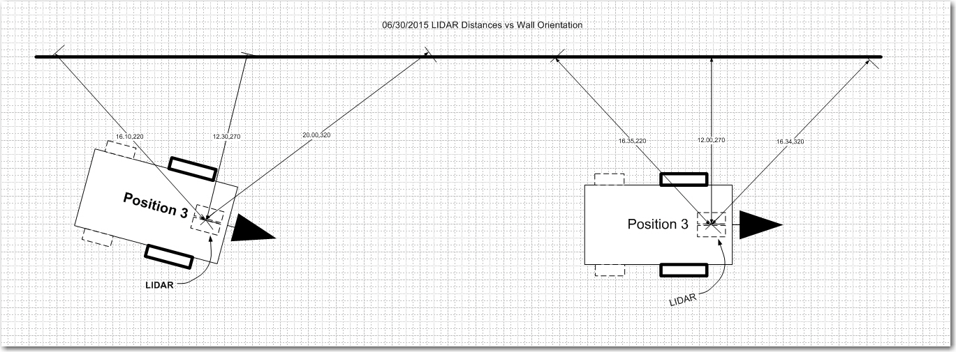
LIDAR distance measurements to a nearby long wall

Test methodology:  I placed Wall-E about 20 cm from a long clear wall in three different orientations; parallel to the wall, and then pointed 45 degrees away from the wall, and then 45 degrees toward the wall.  For each orientation I allowed Wall-E to fill the EEPROM with  spinning LIDAR data, which was subsequently retrieved and plotted for analysis.

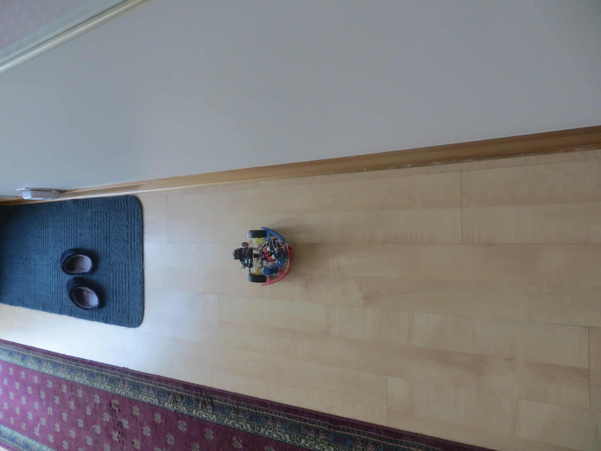
The LIDAR Field Test Area. Note the dreaded stealth  slippers lurking in the background

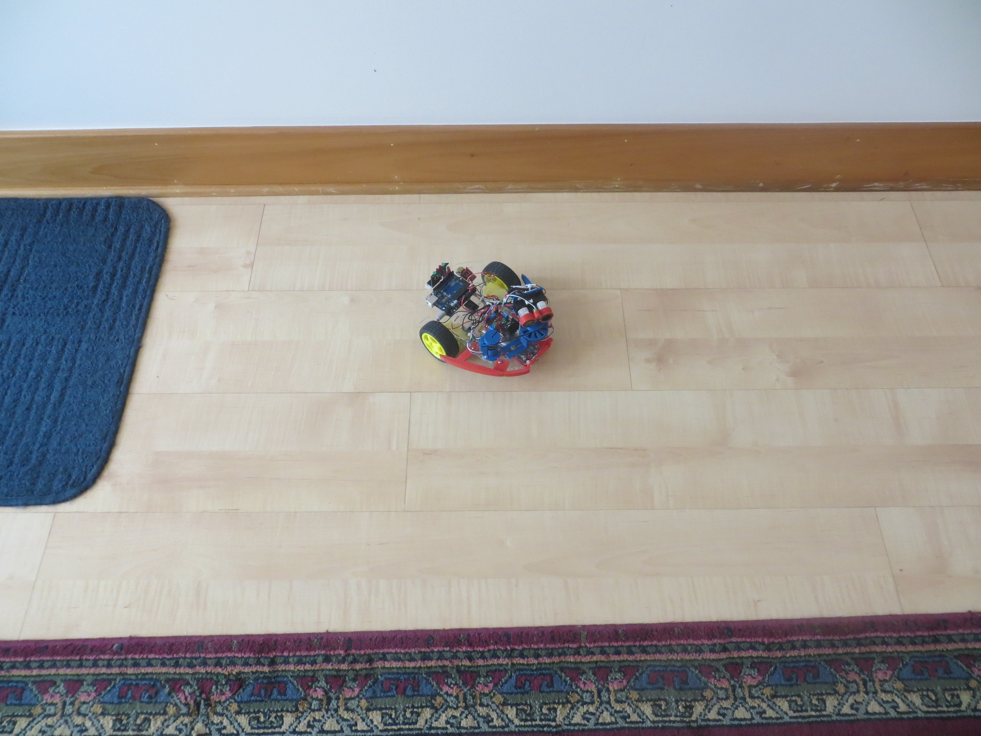
Wall-E oriented at approximately 45 degrees nose-out

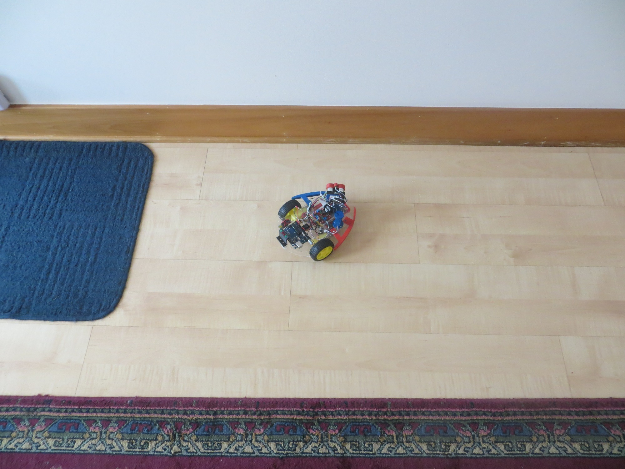
Wall-E oriented at approximately 45 degrees nose-in

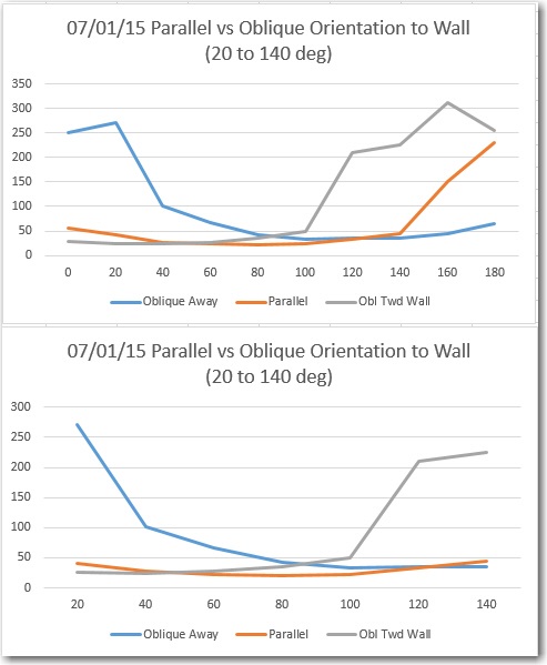
Excel plots of the three orientations. Note the anti-symmetric behavior of the nose-in and nose-out plots, and the symmetric behavior of the parallel case

In each case, data was captured every 20 degrees, but the lower plot above shows only the three data points on either side of the 80-degree datapoint.  In the lower plot,  there are clear differences in the behavior for the three orientation cases.  In the parallel case, the recorded distance data is indeed very symmetric as expected, with a minimum at the 80 degree datapoint.   In the other two cases the data shows anti-symmetric behavior with respect to each other, but unsymmetric with respect to the 20-to-140 plot range.

My original theory was that I could look at one or two datapoints on either side of the directly abeam datapoint (the ’80 degree’ one in this case) and determine the orientation of the robot relative to the wall.  If the off-abeam datapoints were equal or close to equal, then the robot must be oriented parallel.  If they differed sufficiently, then the robot must be nose-in or nose-out.  Nose-in or nose-out conditions would produce a correcting change in wheel speed commands.  The above plots appear to support this theory, but also offer a potentially easier way to make the orientation determination.  It looks like I could simply search through the 7 datapoints from 20 to 140 degrees for the minimum value.  If this value occurs at a datapoint less than 80 degrees, then the robot is nose-in; if more than 80 degrees it is nose-out.  If the minimum occurs right at 80 degrees, it is parallel.  This idea also offers a natural method of controlling the amount of correction applied to the wheel motors – it can be proportional to the minimum datapoint’s distance from 80 degrees.

Of course, there are still some major unknowns and potential ‘gotchas’ in all this.

• First and foremost, I don’t know whether the current measurement rate (approximately two revolutions per second) is fast enough for successful wall following at reasonable forward speeds. It may be that I have to slow Wall-E to crawl to avoid running into the wall before the next correction takes effect.
• Second, I haven’t yet addressed how to negotiate obstacles; it’s all very well to follow a wall, but what to do at the end of a hall, or when going by an open doorway, or …  My tentative plan is to continually search the most recent LIDAR dataset for the maximum distance response (and I can do this now, as the LIDAR doesn’t suffer from the same distance limitations as the acoustic sensors), and try to always keep Wall-E headed in the direction of maximum open space.
• Thirdly, is Wall-E any better off now than before with respect to detecting and recovering from ‘stuck’ conditions.  What happens when (not if!) Wall-E is attacked by the dreaded stealth slippers again?  Hopefully, the combination of the LIDAR’s height above Wall-E’s chassis and it’s much better distance (and therefore, speed) measurement capabilities will allow  a much more robust obstacle detection and ‘stuck detection’ scheme to be implemented.

Stay tuned!

Frank